| Image Segmentation |  |
Section Contents
- Computing Superpixels
- Constructing the Region Adjacency Graph and its Feature Maps
- Perform Hierarchical Clustering
The complete code of the example described here can be found in graph_agglomerative_clustering.cxx.
Computing Superpixels
Hierarchical or agglomerative clustering can be applied either to the pixels directly by using a vigra::GridGraph, or on an initial oversegmentation into superpixels whose region adjacency graph is represented in a vigra::AdjacencyListGraph. We describe the second variant here, as it offers more possibilities, but the first works essentially in the same way.
Before computing superpixels, it is useful to transform the data from the RGB colorspace into the Lab colorspace, because distances in the Lab space are perceptually more meaningful:
VIGRA offers two superpixel algorithms: watersheds and SLIC superpixels. We use the watershed algorithm here, see slicSuperpixels() for more information on the alternative. To run the watershed algorithm, we first need an edge indicator (i.e. an image with big values along edges and small values elsewhere) like the gradient magnitude:
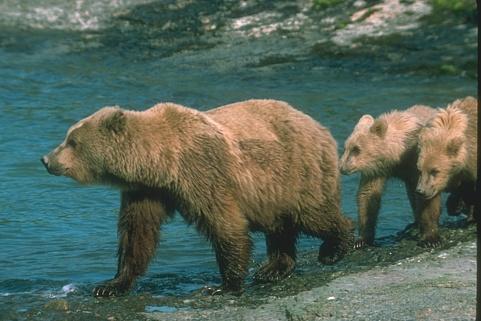
input image | 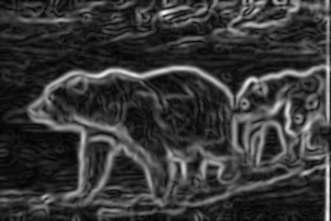
gradient magnitude |
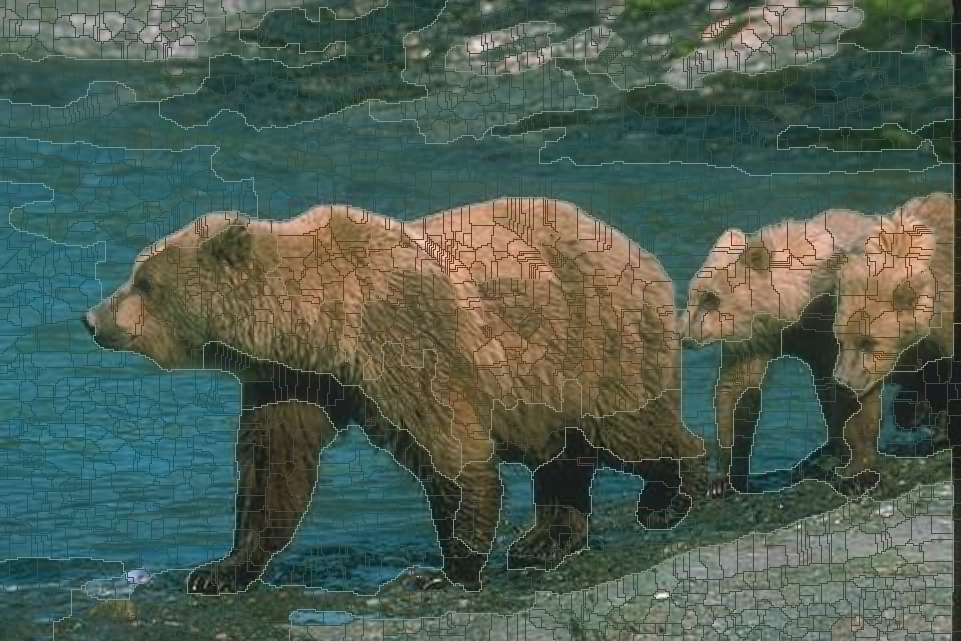
The watershed algorithm initiates a superpixel at every local minimum of the gradient image and then grows these seeds along increasing gradients until they meet at the gradient ridges (called "watersheds" because we can interpret the gradient as the altitude of a landscape) which partly correspond to true image edges, but are also located elsewhere. The goal of the subsequent hierarchical clustering is to identify the true edges and delete the spurious ones. The superpixels are represented in a label image that assigns the superpixel ID to every pixel. To visualize the superpixels, it is useful to display the watershed lines as an overlay on an enlarged version of the input image (Enlarging the image is necessary because the watersheds are actually between pixels, i.e. at half-integer coordinates. Doubling maps these to odd-valued coordinates in the enlarged image, so that rounding is avoided.). In this example, we use the fast union-find watershed algorithm, which is also available in a parallel version in function unionFindWatershedsBlockwise():
Constructing the Region Adjacency Graph and its Feature Maps
Next, we invoke makeRegionAdjacencyGraph() to construct the region adjacency graph (RAG) of the superpixels. This function takes any graph along with a connected components labeling and creates a new graph that has exactly one node per connected component, and nodes are connected by an edge whenever the corresponding components are neighbors in the original graph, i.e. the original graph contains at least one edge with one end point in the first and the other in the second component. In general, each pair of components has several edges with this property, and all of them are mapped onto a single edge in the RAG. To keep track of this mapping, makeRegionAdjacencyGraph() accepts an additional parameter affiliatedEdges, which is a map from edge IDs in the RAG to vectors of edge IDs in the original graph. In our case, the input graph is a vigra::GridGraph whose labeling is stored in the labelArray, and the output graph is a vigra::AdjacencyListGraph. The mapping affiliatedEdges is best constructed by using embedded types of these graph classes:
Note that VIGRA's graph classes conform to the elegant API defined in the LEMON Graph Library. Although VIGRA doesn't use LEMON's implementation of this API, it is worth reading their tutorial because VIGRA's graph classes behave in exactly the same way.
To control agglomerative clustering, i.e. to define the order in which edges are contracted and nodes merged, we need some features that describe the dissimilarity of superpixels. The more dissimilar two superpixels are, the more likely they will remain separated, i.e. belong to different regions of the final segmentation. We distinguish two kinds of features: edge weights and node features.
Edge weights should be high when two superpixels are separated by an object edge, i.e. when the gradient magnitude along the common superpixel boundary is high. We define the edge weight as the average gradient magnitude along the boundary, i.e. as the average over the grid edges that correspond to the present RAG edge. However, as pointed out earlier, watershed boundaries are located between pixels, i.e. on half-integer coordinates, whereas the gradient has been computed on pixels, i.e. at integer coordinates. We solve this problem by linear interpolation: the gradient of a grid edge is the average gradient of its two end points.
Node features are defined by the average Lab color of each superpixel. Hierarchical clustering will later turn this into a node dissimilarity by computing the Euclidean distance between the average colors of neighboring superpixels, possibly weighted by the superpixels' sizes. To compute these features, we invoke VIGRA's Feature Accumulators framework:
To be understood by hierarchicalClustering(), we must copy the features into node property maps which are compatible with the RAG data structure:
Perform Hierarchical Clustering
Now we have collected all information needed to perform agglomerative clustering. We pass the superpixel adjacency graph and its feature maps to the clustering function, and it returns the cluster assignment in a new property map nodeLabels that assigns to every RAG node the ID of the cluster the node belongs to. Thus, nodeLabels plays exactly the same role for the RAG as labelArray did for the grid graph. Cluster IDs are identical to the node IDs of arbitrarly chosen cluster representatives, i.e. they form a sparse subset of the original IDs.
The details of the clustering algorithm can be customized by the option object vigra::ClusteringOptions. Here, we set the termination criterion numClusters, the relative importance of node features and sizes (beta and wardness) and the norm to be used to compute node feature dissimiliarity. Option objects like this are a common idiom in the VIGRA library, because code readability matters.
Finally, we replace the original superpixel labels in labelArray with the new cluster labels from nodeLabels and visualize the resulting region boundaries, this time with a green overlay on the enlarged input image: